Halo Occupation Distribution (HOD) with OpenCosmo

In this tutorial, we compute the Halo Occupation Distribution (HOD) for hydrodynamic simulations from the SCIDAC suite.

The HOD describes the average number of galaxies hosted by halos as a function of halo mass:

[ \langle N_{\mathrm{gal}} \mid M_{\mathrm{halo}} \rangle ]

We will:

Load halo and galaxy data
Select cluster-scale halos
Count galaxies per halo
Compute and plot the HOD

Data Halo Properties Galaxy Properties

Tasks Query Filter Add Columns Evaluate

import numpy as np
import matplotlib.pyplot as plt
import opencosmo as oc
import astropy.units as u

Load dataset¶

We begin by loading the dataset using OpenCosmo.

# Example placeholders — replace with your actual files
halo_file = "haloproperties/m000p-567.haloproperties.hdf5"
gal_file = "galaxyproperties/m000p-567.galaxyproperties.hdf5"

ds = oc.open(halo_file, gal_file, ignore_empty=False)
print(ds)

Collection of halos with galaxy_properties and halo_properties

Inspect dataset structure¶

Each halo is represented as a structure containing:

halo_properties
galaxy_properties

for halo in ds.halos():
    print(halo.keys())
    break

dict_keys(['halo_properties'])

Select cluster-scale halos¶

mass_cut = 5e13 * u.Msun
ds_filt = ds.filter(oc.col("fof_halo_mass") > mass_cut)

def n_galaxies(galaxy_properties):
    return len(galaxy_properties)

ds_filt = ds_filt.evaluate(n_galaxies)

data = ds_filt["halo_properties"].select(
    "n_galaxies"
).get_data("numpy")

halo_props = ds_filt["halo_properties"].with_new_columns(
    log_mass=oc.col("fof_halo_mass").log10()
)

data = halo_props.select(["n_galaxies", "log_mass"]).get_data("numpy")

logM = np.asarray(data["log_mass"], dtype=float)
ngal_list = np.asarray(data["n_galaxies"], dtype=float)

Compute the HOD¶

We bin halos in log mass and compute the mean number of galaxies per bin.

nbins = 8
bins = np.linspace(logM.min(), logM.max(), nbins + 1)
bin_centers = 0.5 * (bins[:-1] + bins[1:])

inds = np.digitize(logM, bins) - 1

mean_ngal = np.zeros(nbins)
std_ngal = np.zeros(nbins)
counts = np.zeros(nbins)

for i in range(nbins):
    mask = inds == i
    counts[i] = np.sum(mask)

    if counts[i] > 0:
        mean_ngal[i] = np.mean(ngal_list[mask])
        std_ngal[i] = np.std(ngal_list[mask])
    else:
        mean_ngal[i] = np.nan
        std_ngal[i] = np.nan

Check bin populations¶

We inspect how many halos fall into each bin.

print("Counts per bin:", counts)

Counts per bin: [55. 45. 21. 20. 14.  7.  1.  1.]

Plot the HOD¶

min_count = 5
valid = (counts >= min_count) & np.isfinite(mean_ngal)

plt.figure(figsize=(7,5))

plt.errorbar(
    bin_centers[valid],
    mean_ngal[valid],
    yerr=std_ngal[valid] / np.sqrt(counts[valid]),
    fmt='o-',
    capsize=4
)

plt.xlabel(r'$\log_{10}(M_{\rm halo}/M_\odot)$')
plt.ylabel(r'$\langle N_{\rm gal} \mid M_{\rm halo} \rangle$')
plt.title("Halo Occupation Distribution (Clusters)")
plt.grid(True, alpha=0.3)

plt.show()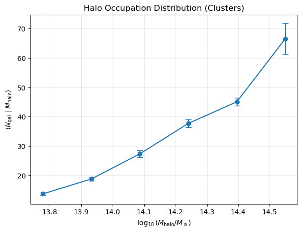

Galaxy counts per halo¶

plt.scatter(logM, ngal_list, alpha=0.3, s=10)

plt.xlabel(r'$\log_{10}(M_{\rm halo}/M_\odot)$')
plt.ylabel(r'$N_{\rm gal}$')
plt.title("Galaxy counts per halo")

plt.grid(True, alpha=0.3)
plt.show()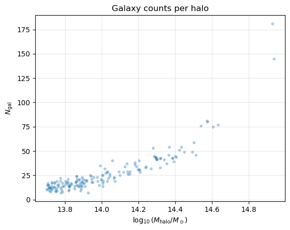

Summary¶

In this tutorial, we:

Loaded halo and galaxy data using OpenCosmo
Selected cluster-scale halos
Counted galaxies per halo
Computed and visualized the Halo Occupation Distribution (HOD)

This workflow can be extended to compare galaxy populations across multiple simulations.

Ideas for Extension

Compare HOD across simulations with different cosmologies or subgrid physics
Add a stellar mass threshold to define “galaxies” more restrictively
Compute separate HODs for central and satellite galaxies
Fit an analytic HOD model (e.g., Zheng et al. 2005) to the results