This tutorial will walk you through the differences between raw galaxies found by DBSCAN, and the galaxies that are reported in the Frontier-E data.
Understand DBSCAN
Investigating stellar masses
Investigating galaxy radii
import opencosmo as oc
import matplotlib.pyplot as plt
from astropy import units as u
from pathlib import Path
data_root = Path("/global/cfs/cdirs/hacc/www/OpenCosmo/understanding-dbscan")
What is DBSCAN?
If you take a look at the columns contained in a galaxy properties file, you may notice that there are columns labeled with DBSCAN. Uncomment the line below and run the cell to see all of the columns in the dataset. Try to find all the columns with this label.
Getting a Feel for Your Dataset
If you don’t know a lot about what is in a dataset you opened, you can use .header, .columns, .descriptions and more to get a better sense of the dataset. Try replacing the line below with data.descriptions to see the difference. See here for even more ways you can quickly get information on your dataset.
ds = oc.open(data_root / 'filtered_galaxy_catalog.hdf5')
# ds.columns
You should have found 3 different columns:
gal_dbscan_mstargal_dbscan_radiusgal_dbscan_count
DBSCAN
In our simulation, galaxies are found by running a clustering algorithm, named DBSCAN (Density-Based Spatial Clustering of Applications with Noise), on the star particles of the simulation. However, most columns in the dataset are not computed from the DBSCAN cluster, and are instead calculated based on the star particles that lie within a given aperture centered on the DBSCAN cluster. The process goes something like this:
Run DBSCAN on all the star particles to find clusters.
Calculate the center of each cluster, taken to be the potential minimum of the star particles
Place an aperture around the center of each cluster, 50 kpc was used in this case
Compute desired quantities.
These columns correspond to a specific type of raw galaxy output from the simulation: the properties of clusters of star particles found by DBSCAN. Let’s look at those columns again and give them proper definitions:
gal_dbscan_mstar: stellar mass from all star particles contained in the clustergal_dbscan_radius: The distance between the center of the cluster and the furthest star particle in the clustergal_dbscan_count: Number of star particles contained in the DBSCAN group.
Making visualizations of the difference between DBSCAN and normal aperture galaxies is difficult and rather involved. Instead, lets just plot these columns in suggestive ways that will help us get a sense of how different the DBSCAN clusters are compared to their aperture counterparts.
Stellar Mass
Let’s start with stellar mass. We can grab the DBSCAN mass column, and the aperture mass column (gal_mass_star), and plot the ratio. Rather than extracting these columns directly and dealing with the subsequent arrays, OpenCosmo can calculate the ratio for us. We first define the operation we want to do using .col() to refer to specific columms (in this case a simple division), and then we feed that operation to .with_new_columns() alongside a name for our new column. We will give it a simple but informative name: “mass_ratio”.
#define the operation
ratio = oc.col('gal_dbscan_mstar') / oc.col('gal_mass_star')

#create new column with OpenCosmo
ds = ds.with_new_columns(mass_ratio = ratio)
With the cell above, OpenCosmo calculated the ratio for us, and now we can simply get the data by using .select() and plot.
#extract ratio
ratio = ds.select('mass_ratio').get_data()

#print ratio range
print('The lowest value of the DBSCAN/Aperture ratio is ', ratio.min(),' and the largest is ', ratio.max())

#plot
plt.hist(ratio, bins = 200)
plt.xlabel('$M_{*,DBSCAN}$ / $M_{*,aperture}$', fontsize = 14)
plt.ylabel('Counts', fontsize = 14)
plt.yscale('log')
plt.xlim(0.5, 11)
plt.show()
The lowest value of the DBSCAN/Aperture ratio is 1.0 and the largest is 11.205097198486328
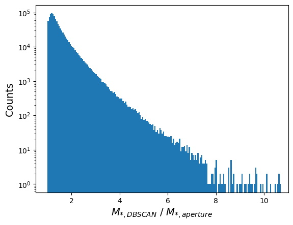
A ratio of 1 means that every particle in the DBSCAN cluster is contained within the aperture. It’s a good sign that most galaxies lie at or around a ratio of 1, implying that the aperture galaxy represents the DBSCAN cluster well. However, we also see ratios can get as large as 11, with hundreds of galaxies at a ratio of 4 or higher.
What causes such large mass discrepancies? What types of galaxies are more likely to have larger DBSCAN masses?
One reason for these large mass ratios is Overlinking, where the DBSCAN algorithm links together multiple galaxies that should be identified separately. This can happen during an active merger, where the boundaries of the two galaxies can get blurred, but it can also happen for massive central galaxies in galaxy clusters. In massive clusters, the Intra-Cluster Light (ICL) can act as a bridge that links multiple galaxies together, if it is dense enough.
One might expect the ratio to be higher for more massive galaxies. To show this, we can look at the mass ratio as a function of galaxy mass. To break the dataset into mass bins we will have to use .filter(). First, you have to define a filtering criterion, using .col() to refer to specific columns, then pass it to OpenCosmo.
#define our log bin edges and figure
bins = [11, 11.25, 11.5, 11.75, 12]
fig, axs = plt.subplots(2, 2, figsize=(12, 8))

#filter for each axis
for ind, ax in enumerate(axs.flatten()):

    #define mass bin filter criterion
    mask = (oc.col('gal_mass_star') < 10**bins[ind+1]) & (oc.col('gal_mass_star') > 10**bins[ind])

    #filter and select the mass ratio
    ratio = ds.filter(mask).select('mass_ratio').get_data()

    #plot
    ax.hist(ratio, bins = 200)
    ax.set_xlabel('$M_{*,DBSCAN}$ / $M_{*,aperture}$', fontsize = 14)
    ax.set_ylabel('Counts', fontsize = 14)
    ax.set_title('Log $M_{*,aperture}$ = ' + f'[{bins[ind]}, {bins[ind+1]}]')
    ax.set_yscale('log')
    ax.set_xlim(0.5, 11)

plt.tight_layout()
plt.show()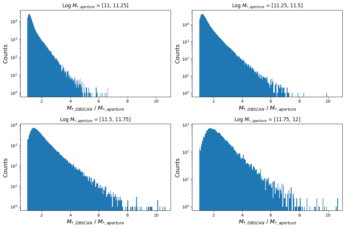
Notice how both the peak and tail of the distribution shifts towards larger mass ratios, thus showing that mass discrepancies get worse at larger masses!
Galaxy Radius
Let’s see if we get similar results by comparing the radius of the DBSCAN cluster to the aperture, which was 50 kpc for this simulation. The process is the same as above, but this time, when we make our new column, we will divide by the aperture.
#make new column
ratio = oc.col('gal_dbscan_radius') / (0.05*u.Mpc)
ds = ds.with_new_columns(radius_ratio = ratio)

#extract column data
ratio = ds.select('radius_ratio').get_data()

#print ratio range
print('The lowest value of the DBSCAN/Aperture ratio is ', ratio.min(),' and the largest is ', ratio.max())

#plot
plt.hist(ratio, bins = 200)
plt.xlabel('$R_{*,DBSCAN}$ / 50 kpc', fontsize = 14)
plt.ylabel('Counts', fontsize = 14)
plt.yscale('log')
plt.show()
The lowest value of the DBSCAN/Aperture ratio is 0.7453400641679764 and the largest is 47.50483512878418
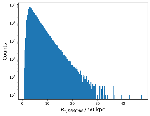
We get a similar result as above! Ratio values below 1 repesent DBSCAN clusters that are fully contained within their aperture, and ratios greater than 1 mean that the cluster extends past the aperture. As before, let’s also look at this plot in different mass bins.
bins = [11, 11.25, 11.5, 11.75, 12]
fig, axs = plt.subplots(2, 2, figsize=(12, 8))
for ind, ax in enumerate(axs.flatten()):

    #filter and get ratio
    mask = (oc.col('gal_mass_star') < 10**bins[ind+1]) & (oc.col('gal_mass_star') > 10**bins[ind])
    ratio = ds.filter(mask).select('radius_ratio').get_data()

    ax.hist(ratio, bins = 200)
    ax.set_xlabel('$R_{*,DBSCAN}$ / 50 kpc', fontsize = 14)
    ax.set_ylabel('Counts', fontsize = 14)
    ax.set_title('Log $M_{*,aperture}$ = ' + f'[{bins[ind]}, {bins[ind+1]}]')
    ax.set_yscale('log')
    ax.set_xlim(0.5, 40)

plt.tight_layout()
plt.show()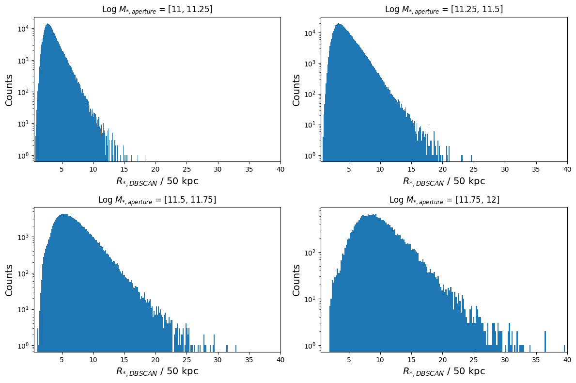
Just like for the mass ratio, the peak and tail shift to higher values as we increase mass. This is also clear evidence of overlinking because the extent of your cluster will be significantly more than a 50 kpc aperture if it contains multiple linked galaxies.
What About gal_dbscan_count?
gal_dbscan_count?Given that the mass of each galaxy comes from summing the mass of its star particles, we will get very similar results if we look at the ratio of particle count. To see if you fully understand this tutorial, make similar plots to the above using this column. You can estimate the number of star particles in the aperture by dividing the total galaxy stellar mass by the median star particle mass. For this simulation, the median star particle mass is . Refer to the documentation if you need help using certain functions!
The takeaway here is that one should be careful when using the properties of very massive galaxies, as particle overlinking may influence the reported mass and size of the galaxy. For most use cases, the effects of overlinking is small and can be ignored, but for more complex analyses it should be taken into account.